Harness the power of AI and ML using Splunk and Amazon SageMaker Canvas

As the scale and complexity of data handled by organizations increase, traditional rules-based approaches to analyzing the data alone are no longer viable. Instead, organizations are increasingly looking to take advantage of transformative technologies like machine learning (ML) and artificial intelligence (AI) to deliver innovative products, improve outcomes, and gain operational efficiencies at scale. Furthermore, the democratization of AI and ML through AWS and AWS Partner solutions is accelerating its adoption across all industries.

For example, a health-tech company may be looking to improve patient care by predicting the probability that an elderly patient may become hospitalized by analyzing both clinical and non-clinical data. This will allow them to intervene early, personalize the delivery of care, and make the most efficient use of existing resources, such as hospital bed capacity and nursing staff.

AWS offers the broadest and deepest set of AI and ML services and supporting infrastructure, such as Amazon SageMaker and Amazon Bedrock, to help you at every stage of your AI/ML adoption journey, including adoption of generative AI. Splunk, an AWS Partner, offers a unified security and observability platform built for speed and scale.

As the diversity and volume of data increases, it is vital to understand how they can be harnessed at scale by using complementary capabilities of the two platforms. For organizations looking beyond the use of out-of-the-box Splunk AI/ML features, this post explores how Amazon SageMaker Canvas, a no-code ML development service, can be used in conjunction with data collected in Splunk to drive actionable insights. We also demonstrate how to use the generative AI capabilities of SageMaker Canvas to speed up your data exploration and help you build better ML models.

Use case overview

In this example, a health-tech company offering remote patient monitoring is collecting operational data from wearables using Splunk. These device metrics and logs are ingested into and stored in a Splunk index, a repository of incoming data. Within Splunk, this data is used to fulfill context-specific security and observability use cases by Splunk users, such as monitoring the security posture and uptime of devices and performing proactive maintenance of the fleet.

Separately, the company uses AWS data services, such as Amazon Simple Storage Service (Amazon S3), to store data related to patients, such as patient information, device ownership details, and clinical telemetry data obtained from the wearables. These could include exports from customer relationship management (CRM), configuration management database (CMDB), and electronic health record (EHR) systems. In this example, they have access to an extract of patient information and hospital admission records that reside in an S3 bucket.

The following table illustrates the different data explored in this example use case.

This post describes an approach with two key components:

• The two data sources are stored alongside each other using a common AWS data engineering pipeline. Data is presented to the personas that need access using a unified interface.
• An ML model to predict hospital admissions (admitted) is developed using the combined dataset and SageMaker Canvas. Professionals without a background in ML are empowered to analyze the data using no-code tooling.

The solution allows custom ML models to be developed from a broader variety of clinical and non-clinical data sources to cater for different real-life scenarios. For example, it can be used to answer questions such as “If patients have a propensity to have their wearables turned off and there is no clinical telemetry data available, can the likelihood that they are hospitalized still be accurately predicted?”

AWS data engineering pipeline

The adaptable approach detailed in this post starts with an automated data engineering pipeline to make data stored in Splunk available to a wide range of personas, including business intelligence (BI) analysts, data scientists, and ML practitioners, through a SQL interface. This is achieved by using the pipeline to transfer data from a Splunk index into an S3 bucket, where it will be cataloged.

The approach is shown in the following diagram.

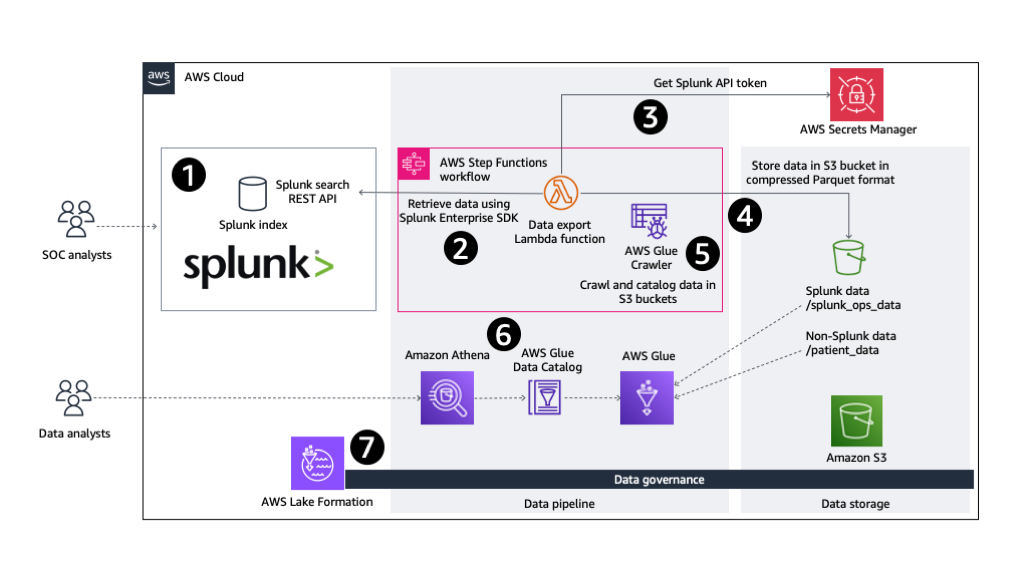
Figure 1: Architecture overview of data engineering pipeline

The automated AWS data pipeline consists of the following steps:

1. Data from wearables is stored in a Splunk index where it can be queried by users, such as security operations center (SOC) analysts, using the Splunk search processing language (SPL). Spunk’s out-of-the-box AI/ML capabilities, such as the Splunk Machine Learning Toolkit (Splunk MLTK) and purpose-built models for security and observability use cases (for example, for anomaly detection and forecasting), can be utilized inside the Splunk Platform. Using these Splunk ML features allows you to derive contextualized insights quickly without the need for additional AWS infrastructure or skills.
2. Some organizations may look to develop custom, differentiated ML models, or want to build AI-enabled applications using AWS services for their specific use cases. To facilitate this, an automated data engineering pipeline is built using AWS Step Functions. The Step Functions state machine is configured with an AWS Lambda function to retrieve data from the Splunk index using the Splunk Enterprise SDK for Python. The SPL query requested through this REST API call is scoped to only retrieve the data of interest.
   • 1. Lambda supports container images. This solution uses a Lambda function that runs a Docker container image. This allows larger data manipulation libraries, such as pandas and PyArrow, to be included in the deployment package.
     2. If a large volume of data is being exported, the code may need to run for longer than the maximum possible duration, or require more memory than supported by Lambda functions. If this is the case, Step Functions can be configured to directly run a container task on Amazon Elastic Container Service (Amazon ECS).
3. For authentication and authorization, the Spunk bearer token is securely retrieved from AWS Secrets Manager by the Lambda function before calling the Splunk /search REST API endpoint. This bearer authentication token lets users access the REST endpoint using an authenticated identity.
4. Data retrieved by the Lambda function is transformed (if required) and uploaded to the designated S3 bucket alongside other datasets. This data is partitioned and compressed, and stored in storage and performance-optimized Apache Parquet file format.
5. As its last step, the Step Functions state machine runs an AWS Glue crawler to infer the schema of the Splunk data residing in the S3 bucket, and catalogs it for wider consumption as tables using the AWS Glue Data Catalog.
6. Wearable data exported from Splunk is now available to users and applications through the Data Catalog as a table. Analytics tooling such as Amazon Athena can now be used to query the data using SQL.
7. As data stored in your AWS environment grows, it is essential to have centralized governance in place. AWS Lake Formation allows you to simplify permissions management and data sharing to maintain security and compliance.

An AWS Serverless Application Model (AWS SAM) template is available to deploy all AWS resources required by this solution. This template can be found in the accompanying GitHub repository.

Refer to the README file for required prerequisites, deployment steps, and the process to test the data engineering pipeline solution.

AWS AI/ML analytics workflow

After the data engineering pipeline’s Step Functions state machine successfully completes and wearables data from Splunk is accessible alongside patient healthcare data using Athena, we use an example approach based on SageMaker Canvas to drive actionable insights.

SageMaker Canvas is a no-code visual interface that empowers you to prepare data, build, and deploy highly accurate ML models, streamlining the end-to-end ML lifecycle in a unified environment. You can prepare and transform data through point-and-click interactions and natural language, powered by Amazon SageMaker Data Wrangler. You can also tap into the power of automated machine learning (AutoML) and automatically build custom ML models for regression, classification, time series forecasting, natural language processing, and computer vision, supported by Amazon SageMaker Autopilot.

In this example, we use the service to classify whether a patient is likely to be admitted to a hospital over the next 30 days based on the combined dataset.

The approach is shown in the following diagram.

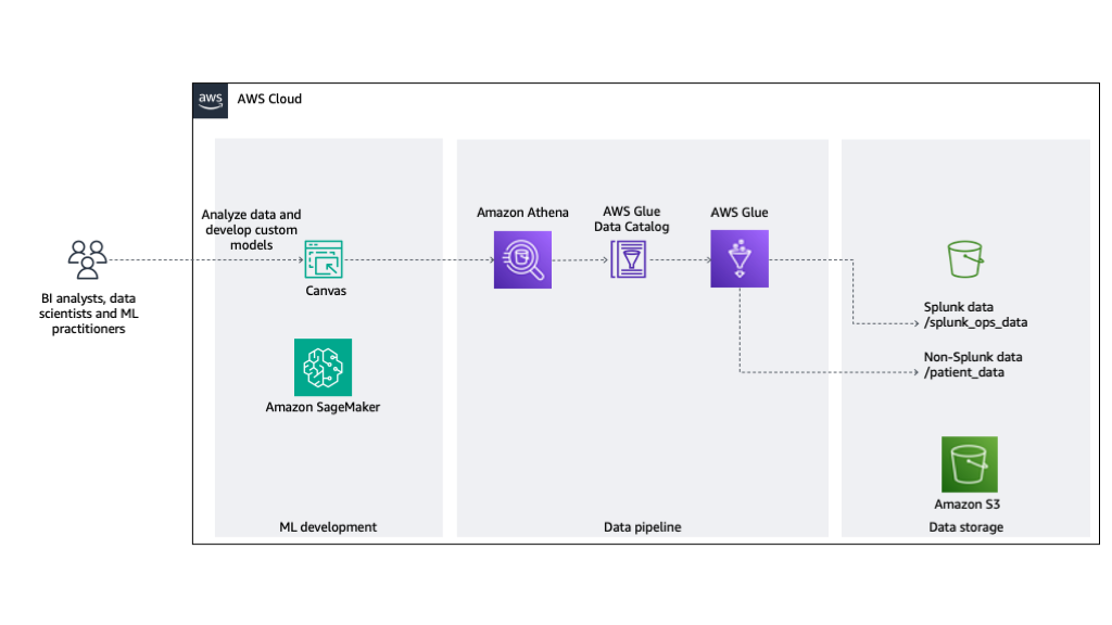
Figure 2: Architecture overview of ML development

The solution consists of the following steps:

1. An AWS Glue crawler crawls the data stored in S3 bucket. The Data Catalog exposes this data found in the folder structure as tables.
2. Athena provides a query engine to allow people and applications to interact with the tables using SQL.
3. SageMaker Canvas uses Athena as a data source to allow the data stored in the tables to be used for ML model development.

Solution overview

SageMaker Canvas allows you to build a custom ML model using a dataset that you have imported. In the following sections, we demonstrate how to create, explore, and transform a sample dataset, use natural language to query the data, check for data quality, create additional steps for the data flow, and build, test, and deploy an ML model.

Prerequisites

Before proceeding, refer to Getting started with using Amazon SageMaker Canvas to make sure you have the required prerequisites in place. Specifically, validate that the AWS Identity and Access Management (IAM) role your SageMaker domain is using has a policy attached with sufficient permissions to access Athena, AWS Glue, and Amazon S3 resources.

Create the dataset

SageMaker Canvas supports Athena as a data source. Data from wearables and patient healthcare data residing across your S3 bucket is accessed using Athena and the Data Catalog. This allows this tabular data to be directly imported into SageMaker Canvas to start your ML development.

To create your dataset, complete the following steps:

1. On the SageMaker Canvas console, choose Data Wrangler in the navigation pane.
2. On the Import and prepare dropdown menu, choose Tabular as the dataset type to denote that the imported data consists of rows and columns.

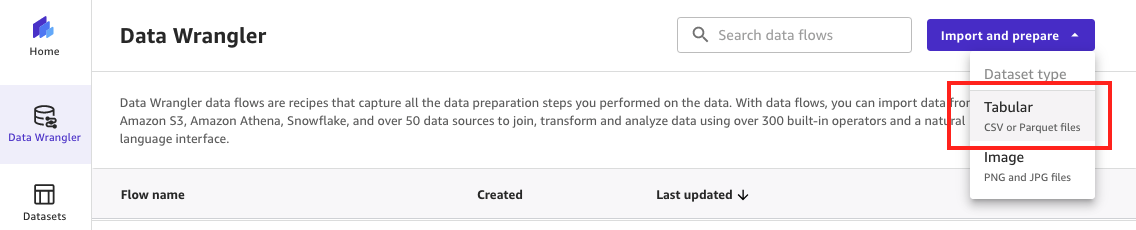
Figure 3: Importing tabular data using SageMaker Data Wrangler

3. For Select a data source, choose Athena.

On this page, you will see your Data Catalog database and tables listed, named patient_data and splunk_ops_data.

4. Join (inner join) the tables together using the user_id and id to create one overarching dataset that can be used during ML model development.
5. Under Import settings, enter unprocessed_data for Dataset name.
6. Choose Import to complete the process.

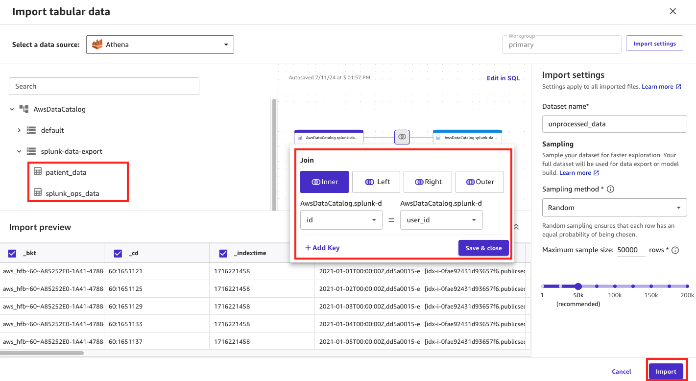
Figure 4: Joining data using SageMaker Data Wrangler

The combined dataset is now available to explore and transform using SageMaker Data Wrangler.

Explore and transform the dataset

SageMaker Data Wrangler enables you to transform and analyze the source dataset through data flows while still maintaining a no-code approach.

The previous step automatically created a data flow in the SageMaker Canvas console which we have renamed to data_prep_data_flow.flow. Additionally, two steps are automatically generated, as listed in the following table.

Before we create additional transform steps, let’s explore two SageMaker Canvas features that can help us focus on the right actions.

Use natural language to query the data

SageMaker Data Wrangler also provides generative AI capabilities called Chat for data prep powered by a large language model (LLM). This feature allows you to explore your data using natural language without any background in ML or SQL. Furthermore, any contextualized recommendations returned by the generative AI model can be introduced directly back into the data flow without writing any code.

In this section, we present some example prompts to demonstrate this in action. These examples have been selected to illustrate the art of the possible. We recommend that you experiment with different prompts to gain the best results for your particular use cases.

Example 1: Identify Splunk default fields

In this first example, we want to know whether there are Splunk default fields that we could potentially exclude from our dataset prior to ML model development.

1. In SageMaker Data Wrangler, open your data flow.
2. Choose Step 2 Data types, and choose Chat for data prep.
3. In the Chat for data prep pane, you can enter prompts in natural language to explore and transform the data. For example:

Prompt: This data has been exported from a Splunk index. Which columns are likely to be Splunk default fields? 
Response: _bkt, _cd, _indextime, _raw, _si, _sourcetype, _time are likely Splunk default fields based on the Summary section showing they are mostly metadata/index fields. 
Prompt: OK. Let's drop _bkt, _cd, _indextime, _raw, _si, _sourcetype, and _time. 
Response: The code drops the columns '_bkt', '_cd', '_indextime', '_raw', '_si', '_sourcetype' and '_time' from the dataframe df using the drop() method.

In this example, the generative AI LLM has correctly identified Splunk default fields that could be safely dropped from the dataset.

4. Choose Add to steps to add this identified transformation to the data flow.

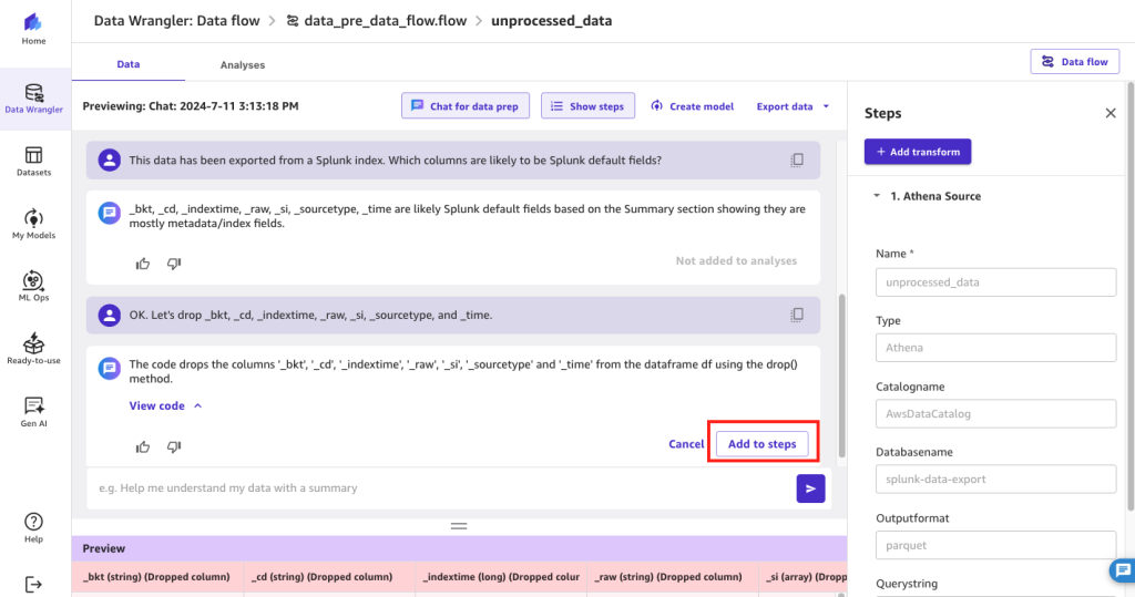
Figure 5: Using SageMaker Data Wrangler’s chat for data prep to identify Splunk’s default fields

Example 2: Identify additional columns that could be dropped

We now want to identify any further columns that could be dropped without being too specific about what we’re looking for. We want the LLM to make the suggestions based on the data, and provide us with the rationale. For example:

Prompt: List out the names of other columns that we should drop before ML development. Give me a list of columns, along with the reasons why. 
Response: The code drops the timestamp, punct, id, index and linecount columns from the dataset. These columns do not contain useful information for machine learning and would add noise to the models.

In addition to the Splunk default fields identified earlier, the generative AI model is now proposing the removal of columns such as timestamp, punct, id, index, and linecount that don’t appear to be conducive to ML model development.

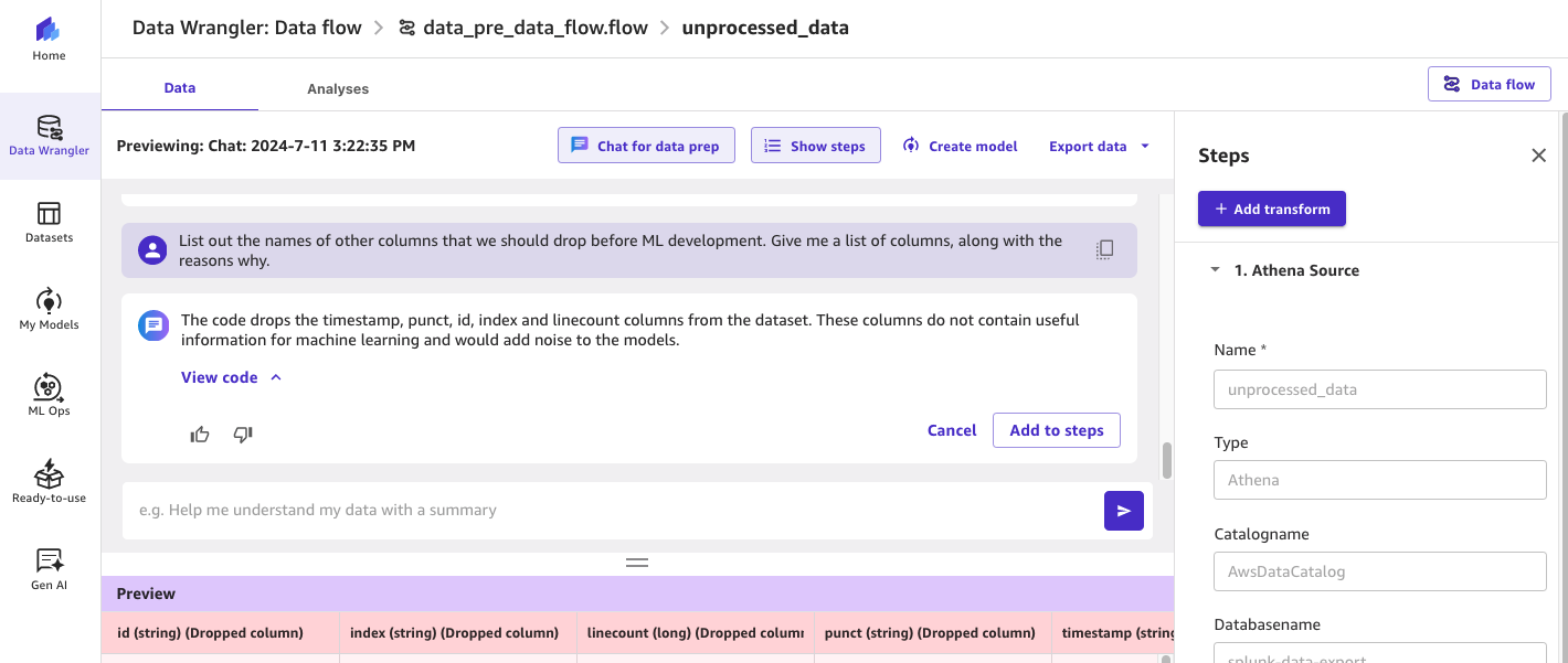
Figure 6: Using SageMaker Data Wrangler’s chat for data prep to identify additional fields that can be dropped

Example 3: Calculate average age column in dataset

You can also use the generative AI model to perform Text2SQL tasks in which you can simply ask questions of the data using natural language. This is useful if you want to validate the content of the dataset.

In this example, we want to know what the average patient age value is within the dataset:

Prompt: What is the average age column of the dataset? 
Response: The average age in the dataset is 67 years.

By expanding View code, you can see what SQL statements the LLM has constructed using its Text2SQL capabilities. This gives you full visibility into how the results are being returned.

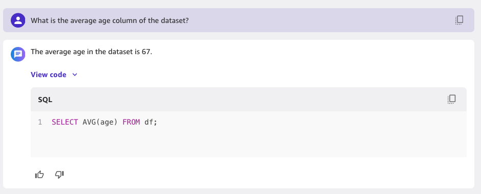
Figure 7: Using SageMaker Data Wrangler’s chat for data prep to run SQL statements

Check for data quality

SageMaker Canvas also provides exploratory data analysis (EDA) capabilities that allow you to gain deeper insights into the data prior to the ML model build step. With EDA, you can generate visualizations and analyses to validate whether you have the right data, and whether your ML model build is likely to yield results that are aligned to your organization’s expectations.

Example 1: Create a Data Quality and Insights Report

Complete the following steps to create a Data Quality and Insights Report:

1. While in the data flow step, choose the Analyses tab.
2. For Analysis type, choose Data Quality and Insights Report.
3. For Target column, choose admitted.
4. For Problem type, choose Classification.

This performs an analysis of the data that you have and provides information such as the number of missing values and outliers.

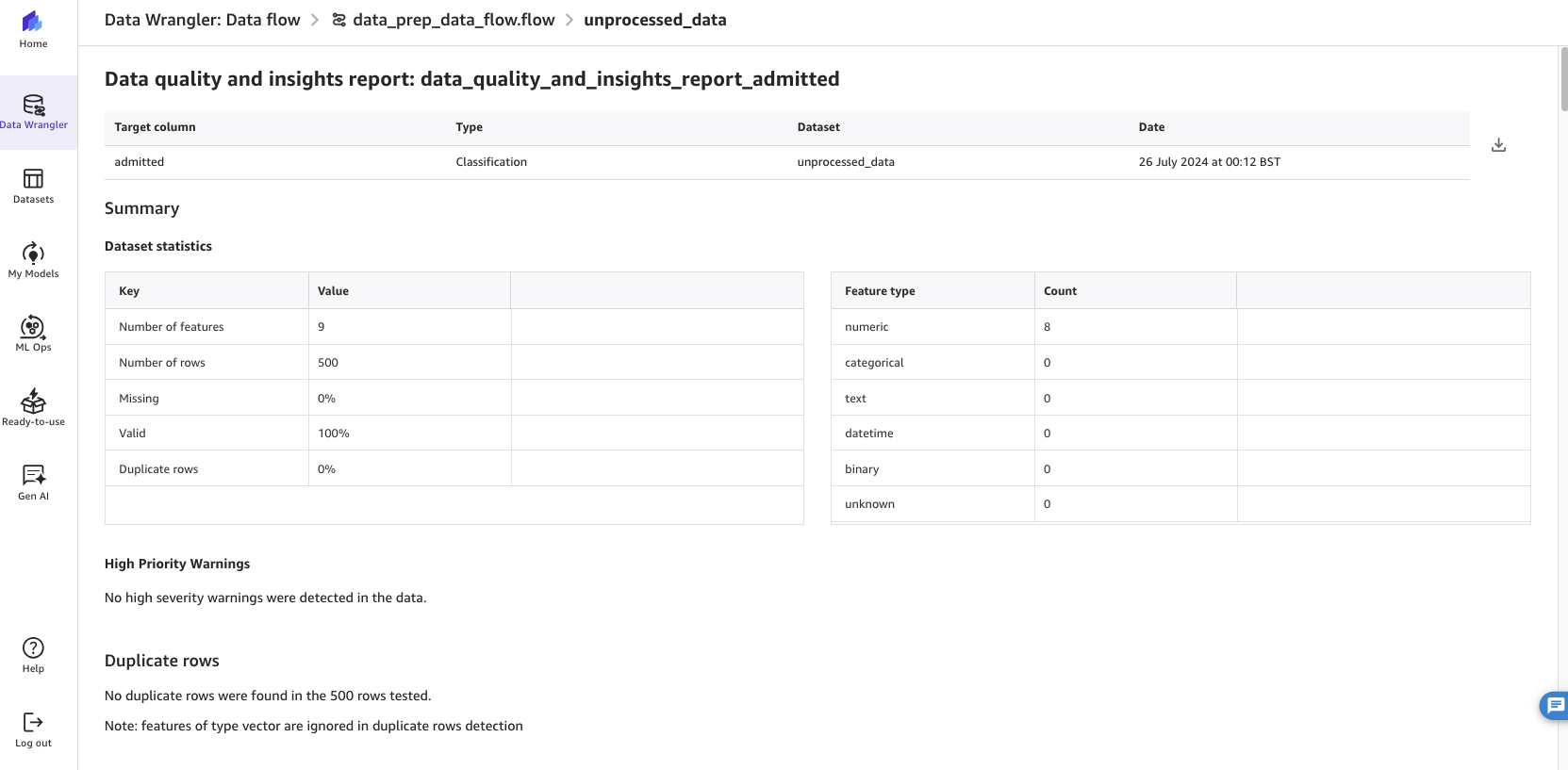
Figure 8: Running SageMaker Data Wrangler’s data quality and insights report

Refer to Get Insights On Data and Data Quality for details on how to interpret the results of this report.

Example 2: Create a Quick Model

In this second example, choose Quick Model for Analysis type and for Target column, choose admitted. The Quick Model estimates the expected predicted quality of the model.

By running the analysis, the estimated F1 score (a measure of predictive performance) of the model and feature importance scores are displayed.

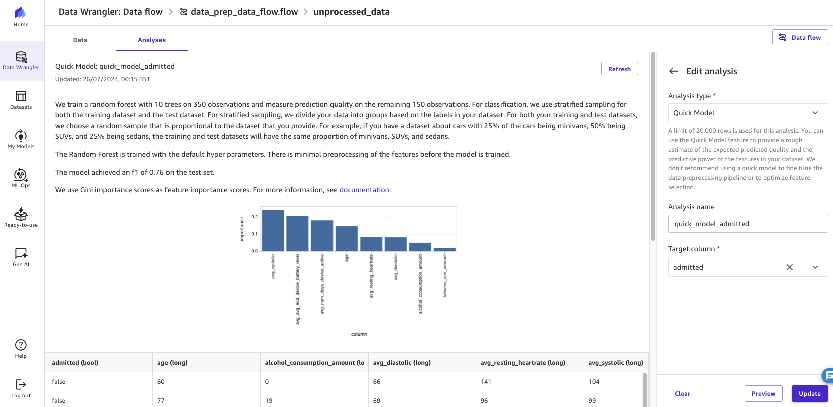
Figure 9: Running SageMaker Data Wrangler’s quick model feature to assess the potential accuracy of the model

SageMaker Canvas supports many other analysis types. By reviewing these analyses in advance of your ML model build, you can continue to engineer the data and features to gain sufficient confidence that the ML model will meet your business objectives.

Create additional steps in the data flow

In this example, we have decided to update our data_prep_data_flow.flow data flow to implement additional transformations. The following table summarizes these steps.

To create a new transform, view the data flow, then choose Add transform on the last step.

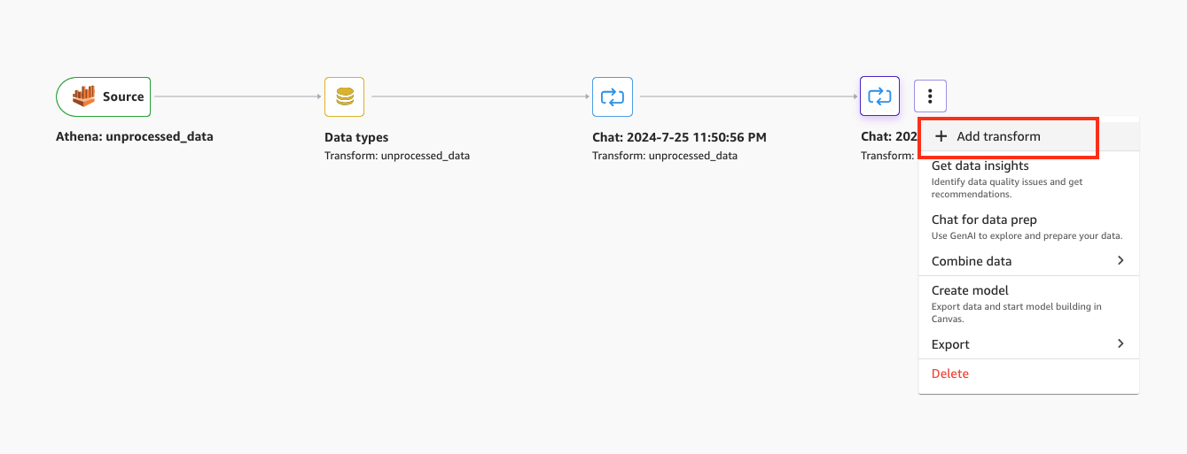
Figure 10: Using SageMaker Data Wrangler to add a transform to a data flow

Choose Add transform, and proceed to choose a transform type and its configuration.

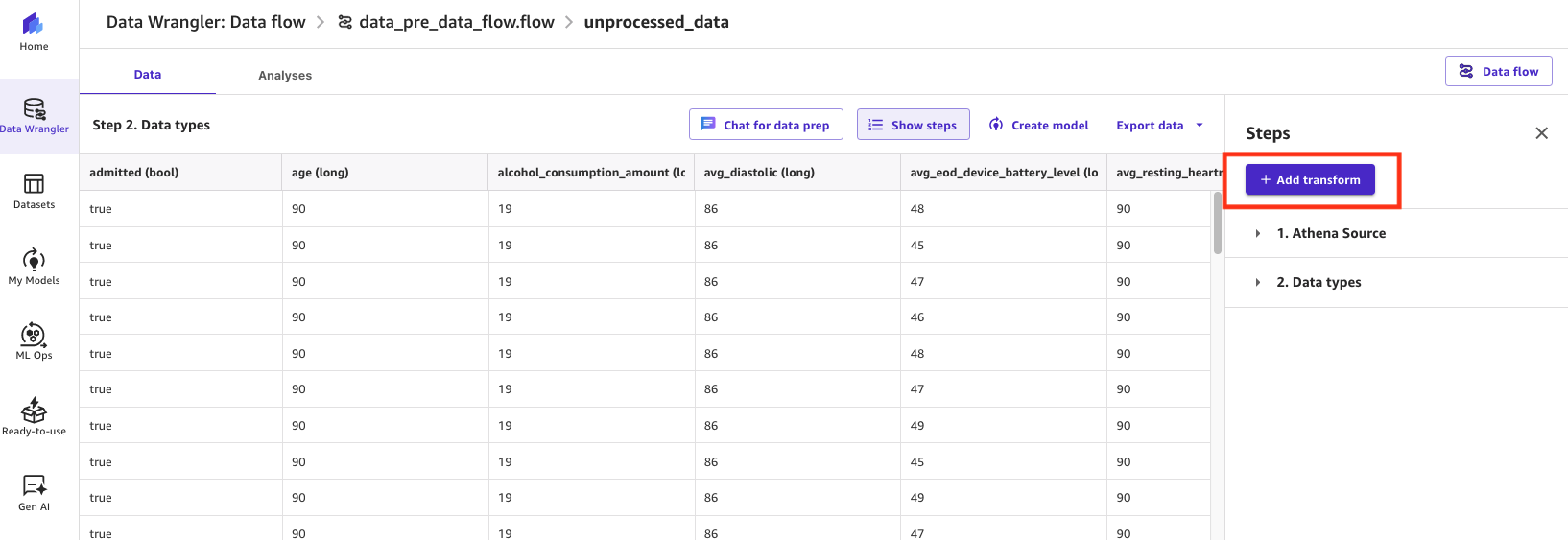
Figure 11: Using SageMaker Data Wrangler to add a transform to a data flow

The following screenshot shows our newly updated end-to-end data flow featuring multiple steps. In this example, we ran the analyses at the end of the data flow.

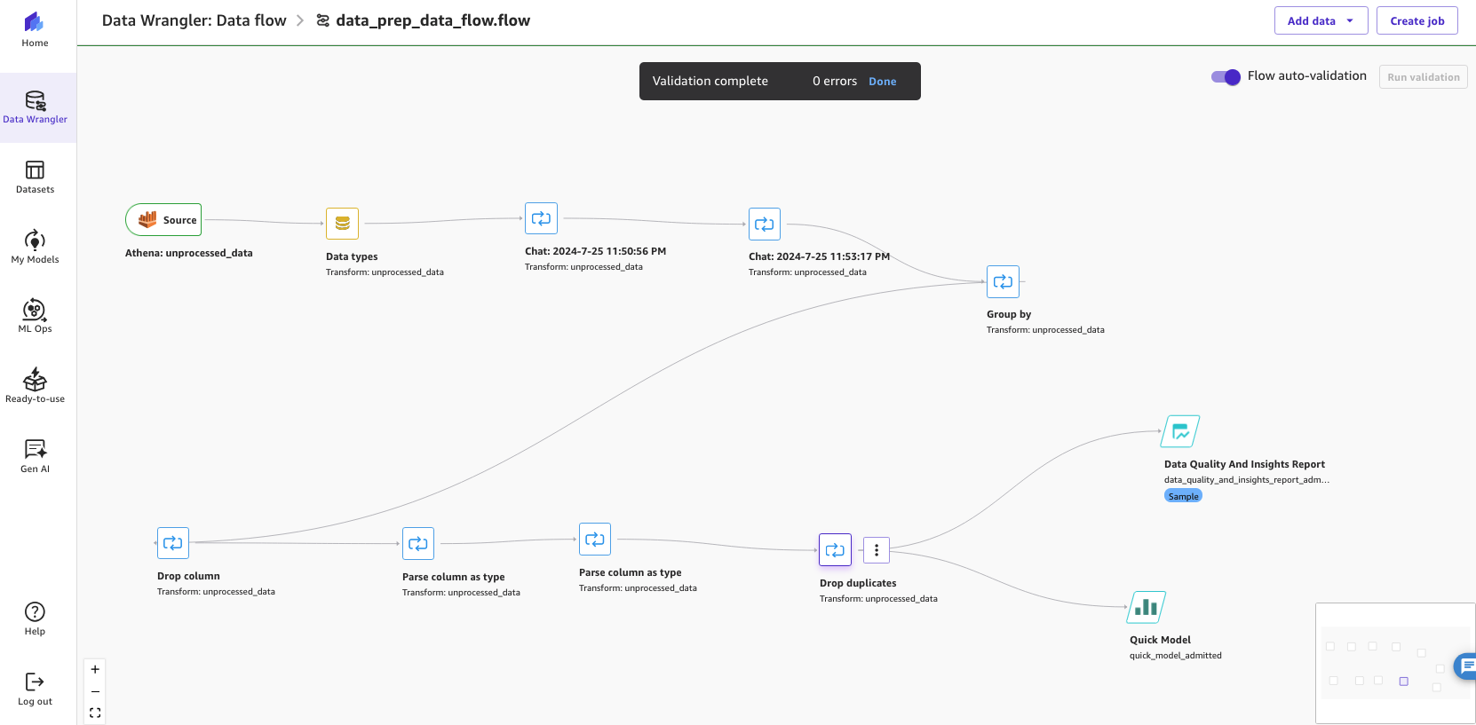
Figure 12: Showing the end-to-end SageMaker Canvas Data Wrangler data flow

If you want to incorporate this data flow into a productionized ML workflow, SageMaker Canvas can create a Jupyter notebook that exports your data flow to Amazon SageMaker Pipelines.

Develop the ML model

To get started with ML model development, complete the following steps:

1. Choose Create model directly from the last step of the data flow.

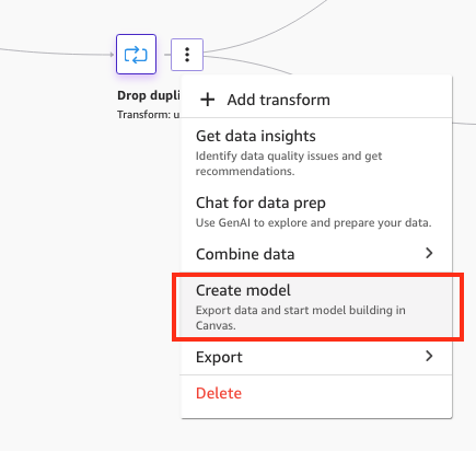
Figure 13: Creating a model from the SageMaker Data Wrangler data flow

2. For Dataset name, enter a name for your transformed dataset (for example, processed_data).
3. Choose Export.

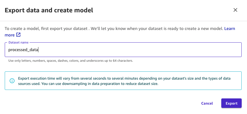
Figure 14: Naming the exported dataset to be used by the model in SageMaker Data Wrangler

This step will automatically create a new dataset.

4. After the dataset has been created successfully, choose Create model to begin the ML model creation.

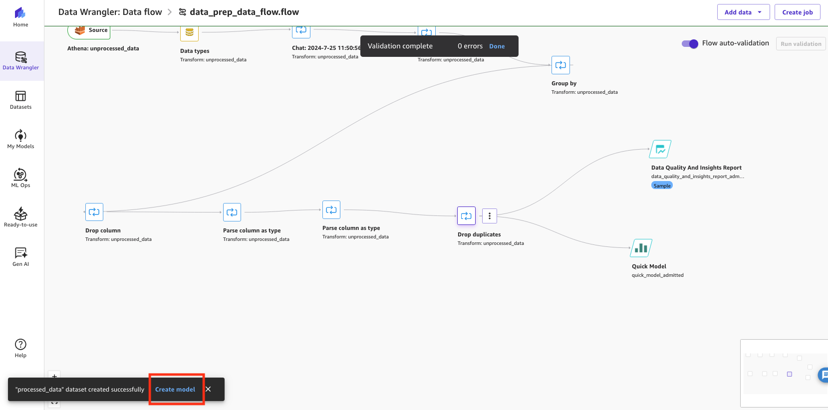
Figure 15: Creating the model in SageMaker Data Wrangler

5. For Model name, enter a name for the model (for example, my_healthcare_model).
6. For Problem type, select Predictive analysis.
7. Choose Create.

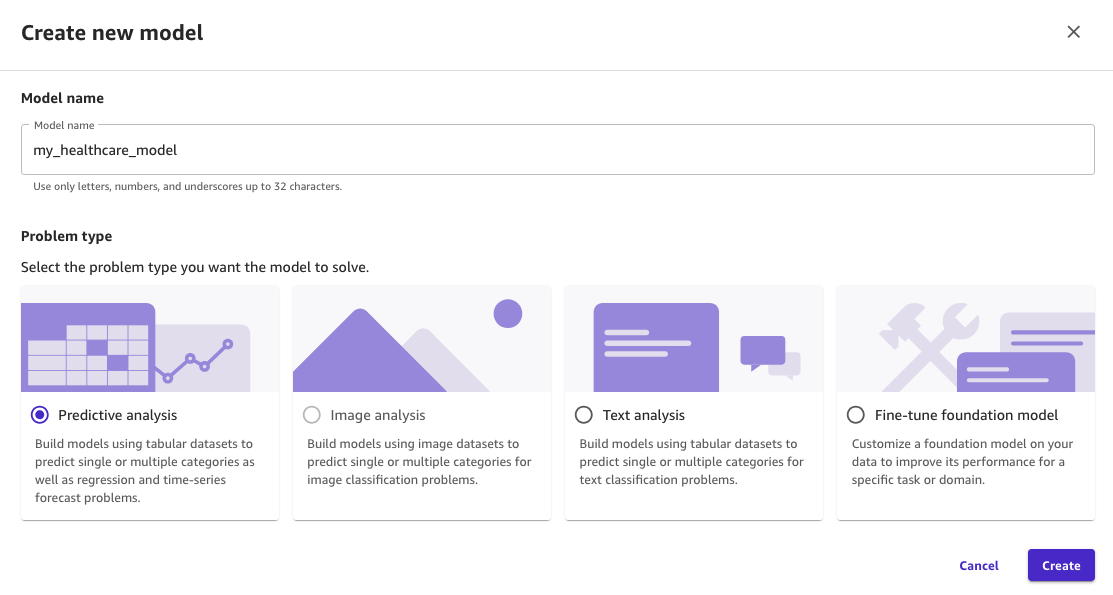
Figure 16: Naming the model in SageMaker Canvas and selecting the predictive analysis type

You are now ready to progress through the Build, Analyze, Predict, and Deploy stages to develop and operationalize the ML model using SageMaker Canvas.

8. On the Build tab, for Target column, choose the column you want to predict (admitted).
9. Choose Quick build to build the model.

The Quick build option has a shorter build time, but the Standard build option generally enjoys higher accuracy.

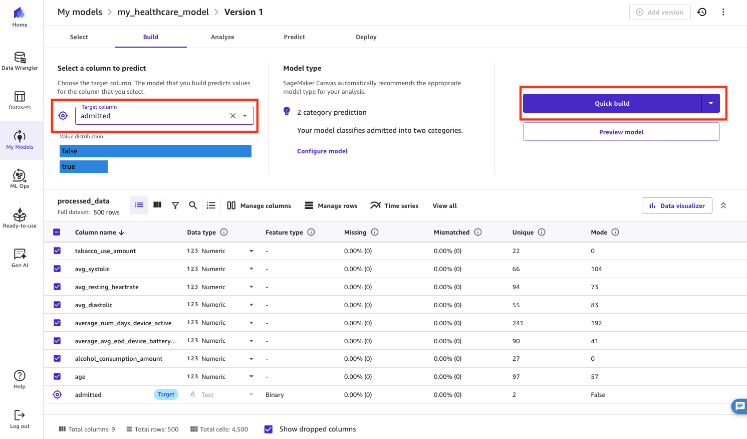
Figure 17: Selecting the target column to predict in SageMaker Canvas

After a few minutes, on the Analyze tab, you will be able to view the accuracy of the model, along with column impact, scoring, and other advanced metrics. For example, we can see that a feature from the wearables data captured in Splunk—average_num_days_device_active—has a strong impact on whether the patient is likely to be admitted or not, along with their age. As such, the health-tech company may proactively reach out to elderly patients who tend to keep their wearables off to minimize the risk of their hospitalization.

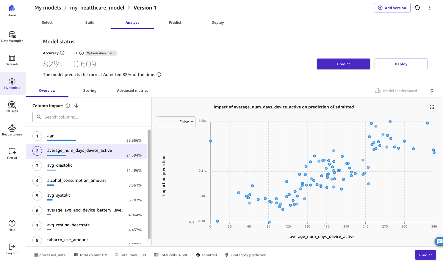
Figure 18: Displaying the results from the model quick build in SageMaker Canvas

When you’re happy with the results from the Quick build, repeat the process with a Standard build to make sure you have an ML model with higher accuracy that can be deployed.

Test the ML model

Our ML model has now been built. If you’re satisfied with its accuracy, you can make predictions using this ML model using net new data on the Predict tab. Predictions can be performed either using batch (list of patients) or for a single entry (one patient).

Experiment with different values and choose Update prediction. The ML model will respond with a prediction for the new values that you have entered.

In this example, the ML model has identified a 64.5% probability that this particular patient will be admitted to hospital in the next 30 days. The health-tech company will likely want to prioritize the care of this patient.

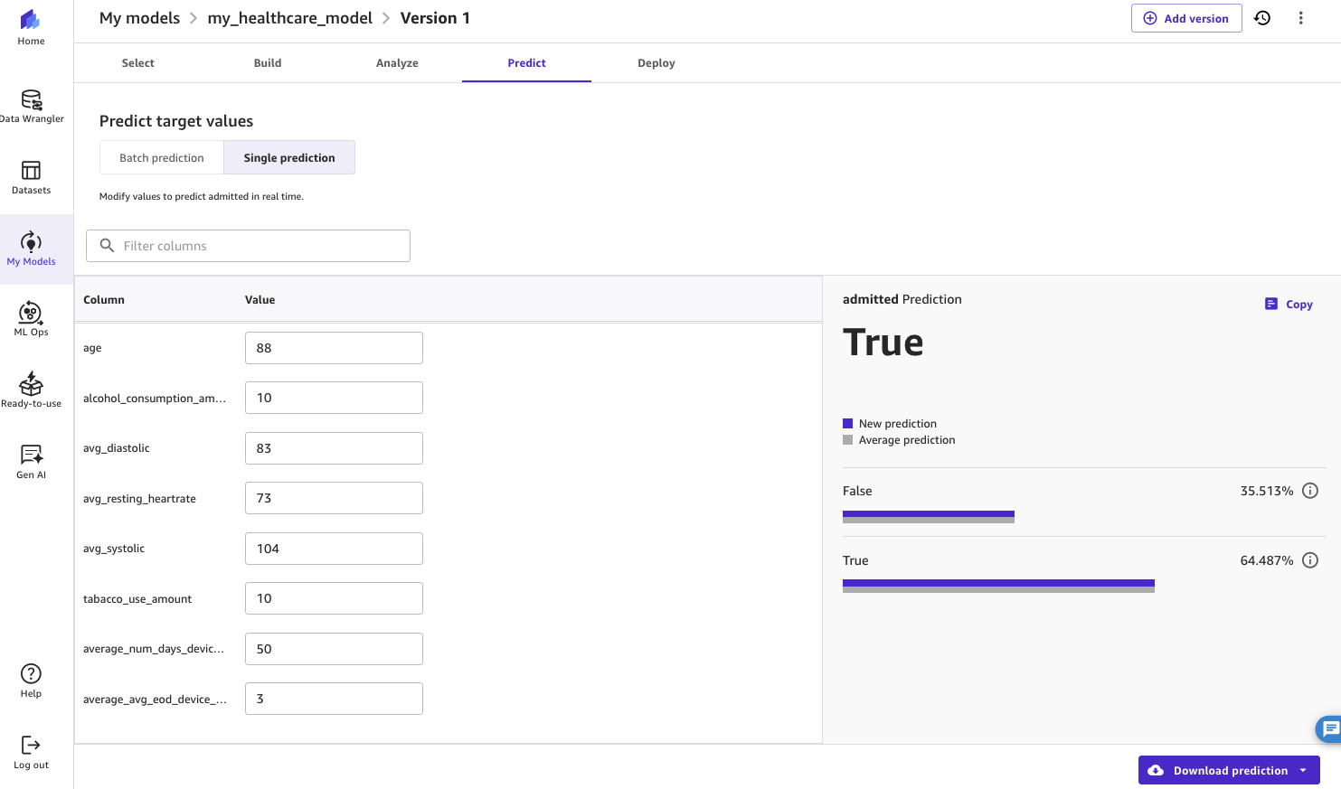
Figure 19: Displaying the results from a single prediction using the model in SageMaker Canvas

Deploy the ML model

It is now possible for the health-tech company to build applications that can use this ML model to make predictions. ML models developed in SageMaker Canvas can be operationalized using a broader set of SageMaker services. For example:

To deploy the ML model, complete the following steps:

1. On the Deploy tab, choose Create Deployment.
2. Specify Deployment name, Instance type, and Instance count.
3. Choose Deploy to make the ML model available as a SageMaker endpoint.

In this example, we reduced the instance type to ml.m5.4xlarge and instance count to 1 before deployment.

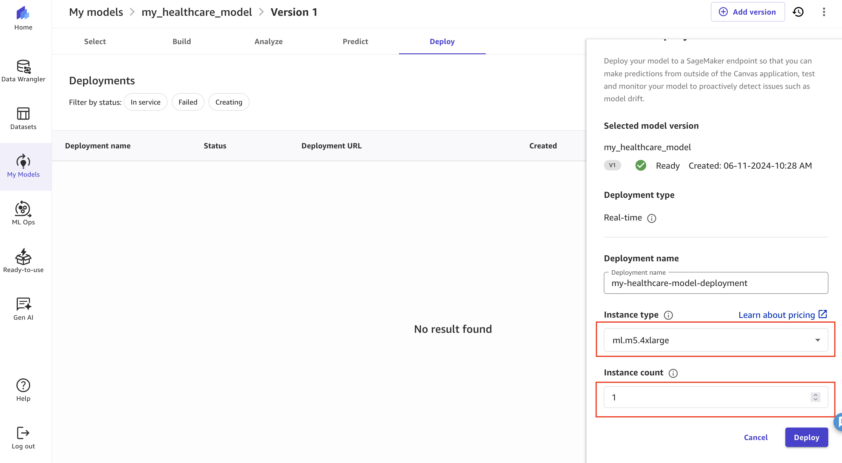
Figure 20: Deploying the using SageMaker Canvas

At any time, you can directly test the endpoint from SageMaker Canvas on the Test deployment tab of the deployed endpoint listed under Operations on the SageMaker Canvas console.

Refer to the Amazon SageMaker Canvas Developer Guide for detailed steps to take your ML model development through its full development lifecycle and build applications that can consume the ML model to make predictions.

Clean up

Refer to the instructions in the README file to clean up the resources provisioned for the AWS data engineering pipeline solution.

SageMaker Canvas bills you for the duration of the session, and we recommend logging out of SageMaker Canvas when you are not using it. Refer to Logging out of Amazon SageMaker Canvas for more details. Furthermore, if you deployed a SageMaker endpoint, make sure you have deleted it.

Conclusion

This post explored a no-code approach involving SageMaker Canvas that can drive actionable insights from data stored across both Splunk and AWS platforms using AI/ML techniques. We also demonstrated how you can use the generative AI capabilities of SageMaker Canvas to speed up your data exploration and build ML models that are aligned to your business’s expectations.

Learn more about AI on Splunk and ML on AWS.

About the Authors

Alan Peaty is a Senior Partner Solutions Architect, helping Global Systems Integrators (GSIs), Global Independent Software Vendors (GISVs), and their customers adopt AWS services. Prior to joining AWS, Alan worked as an architect at systems integrators such as IBM, Capita, and CGI. Outside of work, Alan is a keen runner who loves to hit the muddy trails of the English countryside, and is an IoT enthusiast.

Brett Roberts is the Global Partner Technical Manager for AWS at Splunk, leading the technical strategy to help customers better secure and monitor their critical AWS environments and applications using Splunk. Brett was a member of the Splunk Trust and holds several Splunk and AWS certifications. Additionally, he co-hosts a community podcast and blog called Big Data Beard, exploring trends and technologies in the analytics and AI space.

Arnaud Lauer is a Principal Partner Solutions Architect in the Public Sector team at AWS. He enables partners and customers to understand how to best use AWS technologies to translate business needs into solutions. He brings more than 18 years of experience in delivering and architecting digital transformation projects across a range of industries, including public sector, energy, and consumer goods.